 |
|
| $ \LARGE E=\frac {1} {1+\Big(\frac {R} {R_0}\Big)^6} $ | 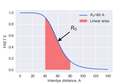 |
$$ \Large {R_0}^6 = \frac{9 \ln 10}{128 \pi^5 N_\text{A}} \frac{\kappa^2 Q_\text{D}}{n^4} J$$
$$ \Large J = \frac{\int f_\text{D}(\lambda) \epsilon_\text{A}(\lambda) \lambda^4 \, d\lambda}{\int f_\text{D}(\lambda) \, d\lambda} = \int \overline{f_\text{D}}(\lambda) \epsilon_\text{A}(\lambda) \lambda^4 \, d\lambda$$
$\kappa = \hat\mu_\text{A} \cdot \hat\mu_\text{D} - 3 (\hat\mu_\text{D} \cdot \hat R) (\hat\mu_\text{A} \cdot \hat R),$ where $\hat\mu_i$ denotes the normalized transition dipole moment of the respective fluorophore, and $\hat R$ denotes the normalized inter-fluorophore displacement.
$$ \Large E = \frac{F_a}{F_a + \gamma F_d} ; \gamma = \frac{\nu_A\Phi_A}{\nu_D\Phi_D}\\ \\ \Large F_D = I_D - B_B - \alpha_{AD}(I_A -B_A)\\ \Large F_A = I_A - B_A - \alpha_{DA}(I_D -B_D) -D{ex} $$
Thus E FRET is sensitive to
- ## $R_0, Q_D$ - depend on dye environment and dye mobility
- ## $\gamma$ - depend on the oplical pathway etc.
$$ \Large R = R_0 \sqrt[6]{\gamma \frac {F_d} {F_a}} $$
from fretbursts import *
from fretbursts.phtools import phrates
sns = init_notebook()
%matplotlib inline
import matplotlib
from fcsfiles import *
# Tweak here matplotlib style
import matplotlib as mpl
mpl.rcParams['font.sans-serif'].insert(0, 'Arial')
mpl.rcParams['font.size'] = 12
%config InlineBackend.figure_format = 'retina'
from IPython.display import display
from bva import bva_sigma_E, bva_sigma_binomial,bva_sigma_binomial_E_asterix
import numpy as np
Loading the data from confocor
## processing confocor files
ch1raw=ConfoCor3Raw('DATA/mono_prox_8%_Ch1.raw')
ch2raw=ConfoCor3Raw('DATA/mono_prox_8%_Ch2.raw')

ch1raw._fh.seek(128)
times = np.fromfile(ch1raw._fh, dtype='<u4', count=-1)
times_acceptor = np.cumsum(times.astype('u8'))

ch2raw._fh.seek(128)
times = np.fromfile(ch2raw._fh, dtype='<u4', count=-1)
times_donor = np.cumsum(times.astype('u8'))
preparing the data for FRET burst analysis
# creating a 2D array of photons
df = np.hstack([np.vstack( [   times_donor, np.zeros(   times_donor.size)] ),
                np.vstack( [times_acceptor,  np.ones(times_acceptor.size)] )]).T

# sorting photons
df_sorted = df[np.argsort(df[:,0])].T

# [0,1,2,3,4,5,6,7] - timestamps
# [0,1,1,0,1,0,1,1] - acceptor mask

d = Data(ph_times_m=[df_sorted[0].astype('int64')], A_em=[df_sorted[1].astype(bool)],
         clk_p=1./ch1raw.frequency, alternated=False, nch=1, fname='MonoNucl_prox')

# That is needed due to issues in FRETbursts package
d.meas_type={}
Background estimation
The recorded stream of timestamps is the result of two processes: one characterized by ahigh count rate, due to fluorescence photons of single molecules crossing the excitation vol-ume, and another characterized by a lower count rate, due to “background counts” originating from
- detector dark counts
- afterpulsing
- out-of-focus molecules
- sample scattering.
The signature of these two types of processes can be observed in the waiting times between two subsequent timestamps. The“tail”of the distribution (a straight line in semi-log scale) corresponds to exponentially-distributed time-delays, indicating that those counts are generated by a Poisson process.
Theory
Three regimes of statistical distributions can be obtained depending on the properties of the light source: Poissonian, super-Poissonian, and sub-Poissonian. Poissonian light can be described by a semi-classical theory in which the light source is modeled as an electromagnetic wave and the atom is modeled according to quantum mechanics.
$$ \large P[N(t)=k] = \frac {e^{-\lambda t} (\lambda t)^k}{k!} \\ $$ Let X be the time between events, than: $$ \large P[X>t]=P[N(t)=0] = \frac {e^{-\lambda t} (\lambda t)^0}{0!}= e^{-\lambda t} \\ \large P[X \leqslant t] = 1 - e^{-\lambda t} \\ \large P[X = t] = \frac {\delta} {\delta t} (1 - e^{-\lambda t})= \lambda e ^ {-\lambda t} $$
d.calc_bg(bg.exp_fit, time_s=60, tail_min_us='auto', F_bg=1.7)
dplot(d, hist_bg, show_fit=True);
dplot(d,timetrace_bg)
plt.show()


Burst searching
The first step of burst analysis is the burst search.
We will use the sliding-window algorithm on all photons. An important variation compared to the classical sliding-windows is that the threshold-rate for burst start is computed as a function of the background and changes when the background changes during the measurement.
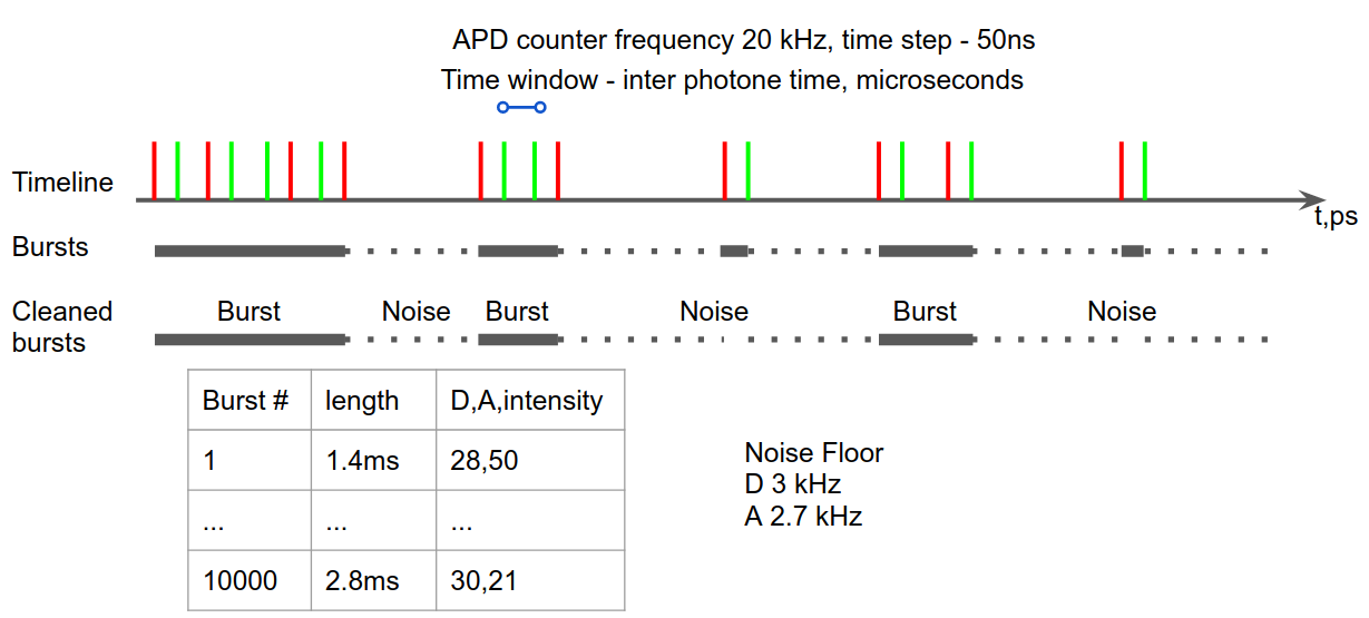
To perform a burst search evaluating the photon rate with:
- m (int) – number of consecutive photons used to compute the photon rate. Typical values 5-20.
- L (int or None) – minimum number of photons in burst.
- F (float) – defines how many times higher than the background rate is the minimum rate used for burst search. Typical values are 3-9. Default 6.
d.burst_search(L=20, m=30, F=6)
dplot(d, hist_fret)

add corrections for instrumental factor and donor fluorescence leakage
d.gamma=0.83
d.leakage=0.19
dplot(d, hist_fret)

Additional thresholding and model fitting
Selecting the bursts in a second step, by applying a minimum burst size criterion, results in a more accurate and unbiased selection. For example, we can select bursts with more than 30 photons (after background, gamma, leakage and direct excitation corrections) and store the result in a new Data() variable ds:
ds = d.select_bursts(select_bursts.size, th1=30)

# defining the model and its boundaries
model = mfit.factory_three_gaussians()
model.set_param_hint('p1_center', value=0.1, min=-0.1, max=0.3)
model.set_param_hint('p2_center', value=0.4, min=0.3, max=0.7)
model.set_param_hint('p3_center', value=0.85, min=0.7, max=1.1)

# Two step fitting
E_fitter = bext.bursts_fitter(ds, 'E', binwidth=0.03)
E_fitter.fit_histogram(model=model, pdf=False, method='nelder')
E_fitter.fit_histogram(model=model, pdf=False, method='leastsq')

# Plotting the resulting histogram
dplot(ds, hist_fret, show_model=True, pdf=False)

# Plotting the timetrace
dplot(ds, timetrace, tmin=0, tmax=1, bursts=True)


Analysing burst lengths
# Select bursts by their E
d_high_fret=ds.select_bursts(select_bursts.E, E1=0.25)
d_low_fret=ds.select_bursts(select_bursts.E, E2=0.25)

# plot timetraces
ax = dplot(d_high_fret, hist_width, bins=(0, 10, 0.2))
dplot(d_low_fret, hist_width, bins=(0, 10, 0.2), ax=ax)
plt.legend(['High-FRET population', 'Low-FRET population'])
plt.show()

Burst Variance Analysis
For a static species, the expected standard deviation due to shot noise, depends only on photon statistics. Any set of consecutive photons will follow a binomial distribution with respect to emission in the donor and acceptor channels.
$$ Pr(k,n,p)= \frac{n!}{k!(n-k)!} p^k (1-p)^{n-k} $$
Assuming no background, the expected standard deviation of $F_A$ should be as variance of binomial distribution
$$ \sigma^2 = np(1-p) $$
$$ p=\frac {F^a}{n}=E $$
$$ \sigma_E = \sqrt\frac{E (1 - E)}{n} $$
To calculate the experimental burstwide standard deviation, we segment each burst $i$, into $M_i$ consecutive (and non overlapping) windows of $n$ photons each,and calculate the standard deviation of all windows within the burst: $$ \sigma_i = \sqrt{\frac{1}{M_i} \sum_{j=1}^{M_i}(\epsilon_{ij} - \mu_i)^2} ; \mu_i = \frac{1}{M_i} \sum_{j=1}^{M_i}(\epsilon_{ij}); \epsilon_{ij}=\frac {F_{ij}^a}{n} $$
To calculate the confidence intervals we will use direct approach $F_{ij}$ are random variables drawn from a binomial distri-bution with n trials and $E^*$ probability of success
$$ \ \sigma = \sqrt{ \sum_{ i(L<E<U)} \sum_{j=1}^{M_i} (\frac{(\frac{F_A^{ij}}{n} - \mu)^2}{\sum M_i}) } ; \ \mu = \sum_{ i(L<E<U)} \sum_{j=1}^{M_i} \frac{\frac{F_A^{ij}}{n} }{\sum M_i} $$
# Preparing the data
ph_d = ds.get_ph_times(ph_sel=Ph_sel(Dex='DAem'))
bursts = ds.mburst[0]
bursts_d = bursts.recompute_index_reduce(ph_d)
Dex_mask = ds.get_ph_mask(ph_sel=Ph_sel(Dex='DAem'))
DexAem_mask = ds.get_ph_mask(ph_sel=Ph_sel(Dex='Aem'))
DexAem_mask_d = DexAem_mask[Dex_mask]

# amount of photons in subburst
plt.figure(figsize=(4.5, 4.5))
n = 7
E_sub_std =bva_sigma_E(n, bursts_d, DexAem_mask_d)
valid = np.isfinite(E_sub_std)
av_e=[]
conf_ivls=[]
B_sub_std=[]


x1=np.arange(0,1.05,0.05)
for i in x1:
    av_e.append(np.average(np.asfarray(E_sub_std)[valid][ (ds.E[0][valid]>=i) & (ds.E[0][valid]<(i+0.05))]))
    B_sub_std.append(bva_sigma_binomial_E_asterix(n, bursts_d, ds.E[0],0.05))

for i in x1:
    conf_ivls.append(np.percentile(np.array(B_sub_std)[:,valid][:,(ds.E[0][valid]>=i) & (ds.E[0][valid]<(i+0.05))].flatten(), 97.5))


x = np.arange(0,1.01,0.01)
y = np.sqrt((x*(1-x))/n)
plt.plot(x, y, lw=2, color='k', ls='--')
#print np.asfarray(E_sub_std)[valid]
im = sns.kdeplot(ds.E[0][valid], np.asfarray(E_sub_std)[valid],
                 shade=True, cmap='Spectral_r', shade_lowest=False, n_levels=20)
plt.fill_between(x1, 0,conf_ivls, facecolor='grey', alpha=0.5,step='post')
#plt.plot(axis,data)
plt.plot(x1+0.025, av_e, lw=2, color='k', ls='',marker='^')
plt.xlim(0,1)
plt.ylim(0,np.sqrt(0.5**2/7)*2)
plt.xlabel('EPR', fontsize=16)
plt.ylabel(r'$\sigma_i$', fontsize=16);
plt.text(0.05, 0.95, '1xN', va='top', fontsize=22, transform=plt.gca().transAxes)
plt.text(0.95, 0.95, '# Bursts: %d' % ds.num_bursts,
         va='top', ha='right', transform=plt.gca().transAxes)
plt.savefig('BVA_di.png', bbox_inches='tight', dpi=600, transparent=False)

def confidence_interval(n, bursts,DexAem_mask_d, bursts_E,e_bin_step, out=None):
    dataframe_mu={}
    dataframe_P={}
    axis=np.arange(0,1,e_bin_step)
    for i in axis:
        dataframe_P[i]=[]

    for burst,e in zip(bursts,bursts_E):
        # clip stuf with nonphysical values
        if e>1:
            e=1
        elif e<0:
            e=0
        e=e_bin_step*(e//e_bin_step) + e_bin_step/2
        bin_=e_bin_step*(e//e_bin_step)
        startlist = range(burst.istart, burst.istop + 2 - n, n)
        stoplist = [i + n for i in startlist]
        burst_p=[]
        for start, stop in zip(startlist, stoplist):
            A_D = DexAem_mask[start:stop].sum()
            P=np.random.binomial(n,e)/float(n)
            burst_p.append(P)
        dataframe_P[bin_].append(np.std(burst_p))

    return dataframe_P

lol=confidence_interval(n, bursts_d, DexAem_mask_d, ds.E[0],0.05)
print lol[0.9]
x=np.linspace(0,140)
R0_=[60]
for R0 in R0_:
    y=1/(1+(x/R0)**6)
    plt.plot(x,y, label='$R_0$=%d A'%R0)

plt.fill_between(x[14:29],0,y[14:29],facecolor='red',alpha=0.5,label='Linear area')
plt.legend()
plt.annotate('$R_0$', xy=(60, 0.5), xytext=(80, 0.7),size=20,
            arrowprops=dict(facecolor='black', shrink=0.01,width=2))

plt.xlabel('Interdye distance, A')
plt.ylabel('FRET E')
plt.savefig('D-Eplot.png')
